Agribusiness Review - Vol. 4 - 1996

Paper 7
ISSN 1442-6951

Food Expenditure Patterns in Urban and Rural Indonesia, 1981 to 1993

Erni Widjajanti
Department of Fisheries, Indonesian Ministry of Agriculture and former student in the Master of Agricultural Business Program, Department of Agricultural Business, University of Adelaide.

and Elton Li
Lecturer, Department of Agricultural Business, University of Adelaide.

The authors wish to thank three anonymous Review referees whose comments improved the paper.
Responsibility is accepted for any remaining errors.

• Abstract
• Introduction
• Objectives
• Table 1: Summary of selected previous studies of food consumption in Indonesia
• Previous studies of food consumption in Indonesia
• Food expenditure patterns, 1981 to 1993
• Allocation of total expenditure between food and non food
• Allocation of expenditure for individual commodities
• Engel curves and income elasticity
• Model specification
• Estimation method and results
• Income elasticity estimates
• Summary and Conclusion
• References
• Footnotes

Abstract

This paper analyses food expenditure patterns in Indonesia with special emphasis on the difference between urban and rural sectors, and on shifts in expenditure patterns over time. Food expenditure patterns in Indonesia vary between urban and rural consumers. Shifts over time in expenditure patterns are also evident. A/though incomes differ between rural and urban areas and have increased over the years, differences in income a/one fail to sufficiently explain variations in food expenditure patterns over time and between rural and urban locations. Rural income elasticity for most food products is higher than for the corresponding urban elasticity. Downward trends in the estimated values of the elasticity for some individual commodities over time are noticeable, with the trends more noticeable for urban areas. Downward trends in income elasticity for cereals are especially pronounced. The relatively high income elasticity for the non-staple food items, both in rural and urban areas, suggest the potential of a large Indonesian market for non-staple food in the future. Notable commodities are meats, eggs and milk; and fruits, which are strong luxuries both in urban and rural areas.

This paper analyses food expenditure patterns in Indonesia with special emphasis on the difference between urban and rural sectors, and on shifts in expenditure patterns over time. Food expenditure patterns in Indonesia vary between urban and rural consumers. Shifts over time in expenditure patterns are also evident. A/though incomes differ between rural and urban areas and have increased over the years, differences in income a/one fail to sufficiently explain variations in food expenditure patterns over time and between rural and urban locations. Rural income elasticity for most food products is higher than for the corresponding urban elasticity. Downward trends in the estimated values of the elasticity for some individual commodities over time are noticeable, with the trends more noticeable for urban areas. Downward trends in income elasticity for cereals are especially pronounced. The relatively high income elasticity for the non-staple food items, both in rural and urban areas, suggest the potential of a large Indonesian market for non-staple food in the future. Notable commodities are meats, eggs and milk; and fruits, which are strong luxuries both in urban and rural areas.

Introduction

In Indonesia, as in most developing countries, food dominates consumers' budgets. In 1993, food constituted over half of consumer expenditure. In rural areas, where about two thirds of the population lived, the food budget share was over 60 per cent. In urban areas, where the average income was higher than the average rural income, the average food budget share was about half of consumer expenditure.

Because of the importance of food, the Indonesian Government places high priority on food and the associated agricultural issues. In the First Twenty-Five-Year Long-Term Development Plan (separated into five year plans called Repelitas, from Repelita 1(1969-1974) to Repelita V (1989-1993), agricultural development was a priority (Morris 1993 ; Piggott et al. 1993 ). In the Fifth Five-Year Development Plan (Repelita V, 1989-1993) the agricultural development objective was to avoid the need for costly food imports to feed the population and to promote agricultural processing, including food processing ( Morris 1993 ). Currently in the Second Twenty-Five-Year Long-Term Development Plan and the Sixth Five-Year Development Plan (Repelita VI, 1994/1995 - 1998/1999), agricultural development is focused towards raising the quantity, quality and diversity of agricultural products, and improving efficiency ( Department of Information 1994 ).

Understanding food expenditure patterns of Indonesia is important because of the significance of food for Indonesia, especially under circumstances of rapid economic growth, rapid population growth, and accelerating urbanisation. Indonesia achieved over 7 per cent economic growth from 1990 to 1994, and this growth is expected to continue. Its population of 198 million in 1995 is projected to increase 46 per cent in 35 years, rising to 290 million in 2030 ( Edwards, MacIntyre and Asra 1995 ). Urban population is projected to increase from 29 per cent of total population in 1992 to 52 per cent in 2020 ( Edwards et al. 1995 ). Increases in population and income mean more food will be required. Just as importantly, changes in food preferences associated with increases in affluence and urbanisation mean that demand for some foods will increase rapidly, while for other foods the increase in demand may be slower. An understanding of historical food expenditure patterns and factors affecting these patterns is necessary for better anticipation of the growth and changes in consumption patterns that are bound to occur. Better anticipation of growth and changes in consumption patterns is of relevance to policy makers and business participants alike.

Objectives

The overall objective of this paper is to analyse the food expenditure patterns in Indonesia with special emphasis on the difference between urban and rural sectors, and shifts in expenditure patterns over time. The analysis is based on secondary SUSENAS 3 data published by the Indonesian Central Bureau of Statistics. Secondary SUSENAS data is published at three year intervals. This paper uses the data published in 1981, 1984, 1987, 1990 and 1993.

Specifically, this paper will focus on the relationship between income and consumption of various food categories. Summary measures of this relationship will be estimated in the form of income elasticity. For each commodity group, the paper aims to assess whether income elasticity is the same for rural and urban areas, and whether there are inter-temporal shifts in this elasticity.

Table 1 : Summary of selected previous studies of food consumption in Indonesia

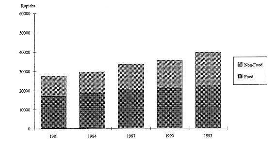
Previous studies of food consumption in Indonesia

Most studies of consumption in Indonesia focus on the staple foods of cereals and cassava. Cereals include rice, corn and wheat. Among the staples, rice is dominant. Most of the studies in Indonesia are based on SUSENAS data, and with few exceptions, use cross-sectional data for one year. Examples of these studies include Sundrum (1977) , Dixon (1979) , Alderman and Timmer (1980) , Daud (1986) , Johnson and Teklu (1988) , Tabor, Altemeier and Adinugroho (1989) , and Rachmat and Erwidodo (1993) . Table 1 presents a summary of the data sources, commodities and elasticity estimates from these studies.

Food expenditure patterns, 1981 to 1993

Introduction

This section highlights developments in food expenditure patterns in Indonesia from 1981 to 1993. All expenditures and prices in this and subsequent sections are adjusted to 1992 market prices by the CPI. Total per capita expenditure (sum of food and non-food expenditure) is used as an approximation for per capita consumer income.

Allocation of total expenditure between food and non food

Figure 1 : Average per capita monthly expenditure for food and non-food in Indonesia at 1992 market prices, 1981 to 1993

Figure 1 shows per capita total expenditure and expenditure allocation between food and non-food for Indonesia for the five years included in the study. Table 2 shows the expenditures in various years relative to the 1981 levels. There has been a steady increase in total expenditure since 1981. Monthly total expenditure per capita increased from Rp 27,603 in 1981 to Rp 39,716 in 1993 (1992 prices), a 44 per cent growth during the twelve year period. Both food and non-food expenditures increased but non-food expenditure increased much faster. Growth in food expenditure from 1981 to 1993 was only 33 per cent, compared to 61 per cent for non-food expenditure.

With food expenditure growing slower than non-food expenditure, its share of expenditure declined. Table 3 shows that the food share declined from 62 per cent in 1981 to 57 per cent in 1993. Food dominated the average consumer's expenditure in Indonesia, however. In each of the five years, food's share of total expenditure in Indonesia was higher than the "world" average of 42 per cent, computed by Selvanathan (1993) for a sample of developed and developing countries.

Table 2 : Increase in average per capita monthly expenditure for food and non-food in Indonesia, 1981 to 1993 (1980 = 1.00)

Source: Biro Pusat Statistik , SUSENAS 1981, 1984, 1987, 1990, 1993.

Table 3 :Food and non-food expenditure shares in Indonesia, 1981 to 1993 (per cent)

Source: Biro Pusat Statistik , SUSENAS 1981, 1984, 1987, 1990, 1993.

Even at this aggregated level of analysis, differences between rural and urban expenditure patterns are noticeable. Table 4 shows the average total expenditure, and food and non-food expenditures, for rural and urban consumers. In 1993, average rural expenditure was only 52 per cent of urban expenditure. This suggests a worsening of the rural-urban income differential since 1981, when average rural expenditure was 56 per cent of urban expenditure. In 1981, rural per capita food expenditure was 70 per cent of urban per capita food expenditure; in 1993 it dropped to 67 per cent. Thus in 1993, an average rural consumer's total expenditure was about half that of an average urban consumer's, but a rural consumer spent about two thirds of what an urban consumer spent on food and about one third on non-food.

Table 4 : Average per capita monthly expenditure for food and non-food in urban and rural areas at 1992 market prices, 1981 to 1993 (Rupiahs)

Source: Biro Pusat Statistik , SUSENAS 1981, 1984, 1987, 1990, 1993.

Table 5 shows urban and rural expenditures in various years relative to the 1981 levels. Per capita urban expenditure increased by 40 per cent from 1981 to 1993 compared to only 30 per cent in rural areas. Over the same period, both per capita non-food and food expenditures increased faster in urban than rural areas. Per capita non-food and food expenditures in urban areas increased by 49 per cent and 31 per cent, compared to only 40 per cent and 25 per cent respectively in rural areas.

Table 5 : Increase in average per capita monthly expenditure for food and non-food in urban and rural areas since 1981 to 1993 (1981 = 1.00)

Source: Biro Pusat Statistik , SUSENAS 1981, 1984, 1987, 1990, 1993.

Table 6 shows that food expenditure shares were much higher in rural areas than in urban areas. In 1993, urban consumers split their expenditure about evenly between food and non-food items, whereas in rural areas consumers spent almost two thirds of their incomes on food. In fact, an average rural consumer's total expenditure is about what an average urban consumer spent on food for every year in the data sample ( Table 4 ).

The food expenditure patterns examined so far are quite consistent with Engel's law that with higher average incomes, a lower fraction of income is spent on food. This is evident both over time and between urban and rural consumers.

Table 6 : Food and non-food expenditure shares in urban and rural areas, 1981 to 1993 (per cent)

Source: Biro Pusat Statistik , SUSENAS 1981, 1984, 1987, 1990, 1993.

For Indonesia as a whole, total expenditure increased 44 per cent from 1981 to 1993. This was accompanied by a decrease of food budget share from 61.5 per cent to 56.9 per cent, a drop of 4.6 percentage points. This is roughly consistent with the strong version of Engel's law, which associates a 10 per cent increase in income with a one percentage point drop in food budget share ( Clements and Chen 1994 ).

Food expenditure share in urban areas decreased from 52.9 per cent in 1981 to 49.8 per cent in 1993, a drop of 3.1 percentage points. During the same period, food expenditure share in rural areas also decreased, from 66.1 per cent to 63.6 per cent, a drop of 2.4 percentage points. From 1981 to 1993, per capita total expenditure increased 40 per cent in urban areas and 30 per cent in rural areas. The decreases in food expenditure share in both rural and urban areas were slightly less than the amount predicted by the strong version of Engel's law. Thus, for this data set, the strong version of the Engel's law appears to hold for Indonesia as a whole but not separately for rural and urban areas.

Allocation of expenditure for individual commodities

Table 7 shows the average per capita expenditures for individual commodities for the five years in the data sample for Indonesia. Table 8 expresses changes m expenditure on each commodity using the 1981 levels as a base. Table 9 shows individual commodity shares as a percentage of total expenditure.

Table 7 : Average per capita monthly expenditure for individual Commodities in Indonesia at 1992 Market Prices, 1981 to 1993 (Rupiahs)

Source: Biro Pusat Statistik , SUSENAS 1981, 1984, 1987,1990, 1993.

For cereals, Table 8 shows that per capita expenditure on cereals in 1993 was 95 per cent of the 1981 level. Expressed as expenditure shares, Table 9 shows that cereals constituted almost 21 per cent of the total in 1981. By 1993, the cereals expenditure share had declined to 14 per cent.

Table 8 : Increase in average per capita monthly expenditure for individual commodities in Indonesia, 1981 to 1993 (1981 = 1.00)

Source: Biro I>usat Statistik , SUSENAS 1981, 1984, 1987,1990, 1993.

Table 9 : Expenditure shares for individual commodities in Indonesia, 1981 to 1993 (per cent)

Source: Biro I>usat Statistik , SUSENAS 1981, 1984, 1987, 1990, 1993.

For all other commodities, there were overall upward trends in per capita expenditures. Commodities with the largest increases in expenditures were prepared food 4 , alcohol, and eggs and milk. Increases in expenditure on prepared food were especially impressive. The expenditure on prepared food in 1993 more than tripled the 1981 level. Table 9 indicates that in 1993, prepared food represented the third largest budget share after cereals and miscellaneous. 5 . The expenditure share for prepared food also increased quite steadily, from 3.4 per cent in 1981 to 7.7 per cent in 1993. Over the same period, the shares for meats, eggs and milk, fruits, and alcohol also increased, whereas for the other commodities the shares declined.

Tables 10, Table 11 and Table 12 are similar to Tables 7, Table 8 and Table 9 respectively but with separate presentation for rural and urban consumers. There are noticeable differences in allocation patterns and the inter-temporal developments of these patterns between rural and urban areas.

Table 10 shows that in 1993, per capita expenditure in urban areas exceeded that in rural areas for every commodity except cereals and cassava. Differences for some commodities were quite substantial. Urban per capita expenditures for meats, eggs and milk, and prepared food, were each over 2.5 times the corresponding rural per capita expenditures. When this is expressed in expenditure share form, Table 12 shows that urban consumers spent 9 per cent of their total expenditure on cereals, compared to 18 per cent for rural consumers. There were also differences in expenditure shares for other commodities but, except for cassava, these were not as drastic as in the case of cereals.

Table 10 : Average per capita monthly expenditure for individual commodities in urban and rural areas at 1992 market prices, 1981-1993 (Rupiahs)

Source: Biro Pusat Statistik , SUSENAS 1981, 1984,1987, 1990, 1993.

Table 11 shows that expenditures on prepared food, alcohol and eggs and milk grew fastest in rural and urban areas. Expenditure on other commodities, except cereals, also increased from 1981 to 1993. For cereals, expenditures declined by 10 per cent in urban areas and 2 per cent in rural areas, from 1981 to 1993.

Table 11 : Growth in average per capita monthly expenditure for individual commodities in urban and rural areas, 1981 to 1993 (1981=1.00)

Source: Biro Pusat Statistik , SUSENAS 1981, 1984, 1987, ~990, 1993.

Engel curves and income elasticity

Introduction

This section focuses on empirical estimation of Engel curves for various food items and aggregates for Indonesia using published SUSENAS data. For each food item, the public shed data reports expenditures for 10 or 11 income groups, and separately for rural and urban areas. This provides the basis for estimating Engel curves, which are cross-sectional relationships between expenditure on an individual good and income level as measured by total expenditures ( Thomas 1987 ).
This section focuses on empirical estimation of Engel curves for various food items and aggregates for Indonesia using published SUSENAS data. For each food item, the public shed data reports expenditures for 10 or 11 income groups, and separately for rural and urban areas. This provides the basis for estimating Engel curves, which are cross-sectional relationships between expenditure on an individual good and income level as measured by total expenditures ( Thomas 1987 ).

Table 12 : Expenditure shares for individual commodities in urban and rural areas, 1981 to 1993 (%)

Source: Biro Pusat Statistik , SUSENAS 1981, 1984, 1987, 1990, 1993.

In cross-sectional budget studies, provided the surveys are completed in a short time-span, prices faced by all households can be regarded as constant, apart from minor variations due to social and regional factors. This allows focus on responses of household demand to variations in income or total expenditure ( Thomas 1987 ). After statistically estimating the Engel curves, the nature of these responses can be summarised by computing income elasticity.

This analysis uses five years of data: 1981, 1984, 1987, 1990 and 1993, with separate consideration of rural and urban areas. Thus, for each food item or food aggregate, there are 10 different Engel curves (one for each year for each of rural and urban consumers). Of interest is whether these Engel curves have remained stable over time and whether these curves are the same for rural and urban areas. To statistically test for this, the five years of data are pooled. Dummy variables are incorporated to allow for different slopes and intercepts for different years and for rural and urban areas. Tests for stability can then be expressed in terms of joint statistical tests on appropriate subsets of the coefficient estimates

For each commodity, income elasticity is computed separately for each year for rural and urban areas. The trends of the elasticity over time and the differences between rural and urban elasticity are assessed.

The estimation covers 12 commodities: cereals, cassava, fish, meats, eggs and milk, vegetables, nuts, fruits, miscellaneous, prepared food, alcohol, and tobacco. In addition, estimation covers aggregated food items and aggregated non-food items.

Model specification

This study uses the semi-log Engel curve:    e = a + b log(c )

Where e is expenditure on the commodity and c is total expenditure or income. 6. Semi-log and double-log forms of the Engel curve have been more successful than other functional forms in cross sectional studies ( Thomas 1987 ). The double-log form has the limitation of constant income elasticity for all levels of income. This disallows a product to change from being a luxury at low-income levels to being a necessity at higher income levels: a characteristic common to many food items. Under the semi-log specification, the income elasticity is b /e . Thus as total expenditure (c) increases, expenditure on the commodity (e) increases, causing income elasticity b /e to decline. This allows a product to be a luxury good at lower income levels and a necessity at higher income levels ( Thomas 1987 ). Since the income elasticity, b /e, vanes at different levels of expenditure (e), the average expenditure level is usually used for e when computing the income elasticity estimate.

Because the data is pooled by year and by urban and rural areas, dummy variables are introduced to allow slope and intercept to vary over the years and between urban and rural areas. Thus, for each item or aggregate, the following expenditure function is estimated:

e = a₀ + a₁ x D₀ + a₂ x D₁ + a₃ x D₂ + a₄ x D₃ + a₅ x D₄

+b₀ xlog(c ) + b₁ x D₀ xlog(c ) + b₂ x D₁ xlog(c )

+b₃ x D₂ xlog(c ) + b₄ x D₃ xlog(c ) + b₅ x D₄ xlog(c )

Where the Greek symbols are the unknown parameters to be estimated, e is expenditure on the commodity, and log(c ) is the natural logarithm of income or total expenditure. The dummy variables are defined as follows:

D₀ = 1, if urban, 0 otherwise
D₁ = 1, if 1981,0 otherwise
D₂ = 1, if 1984,0 otherwise
D₃ = 1, if1987,0 otherwise
D₄ = 1,if 1990, 0 otherwise

With this specification, the Engel curves for individual years and locations (urban versus rural) are:

Thus, testing for homogeneity of Engel curves across years (after accounting for location differences) amounts to testing the null hypothesis:

H₀ : c₀ = c₀ + c₂ = c₀ + c₃ = c₀ + c₄ = c₀ + c₅

b₀ = b₀ + b₂ = b₀ + b₃ = b₀ + b₄ = b₀ + b₅

Or, after simplification:

H₀ : c₂ = c₃ = c₄ = c₅ = b₂ = b₃ = b₄ = b₅ = 0

Similarly, testing for homogeneity of Engel curves across locations (after accounting for inter-temporal differences) amounts to testing the null hypothesis:

H₀ : c₀ = c₀ + c₁ , b₀ = b₀ + b₁

Or more simply:

H₀ : c₁ = b₁ = 0

Estimation method and results

This study uses the Weighted Least Squares (WLS) procedure for estimation. The weights are the proportion of population in each income class. WLS has an advantage over Ordinary Least Squares (OLS) when data used are group averages, as is the case in this study. When a regression uses group averages as data, heteroscedasticity should be expected since group averages computed from larger groups should have smaller sampling variances. WLS corrects for this ( Johnston 1972 ). Intuitively, the WLS procedure gives more importance to observations associated with income classes with larger proportions of population, whereas OLS treats all observations as of equal importance.

Table 13 presents the result of the estimation. The 14 rows of the table present the estimated results for the 14 items and aggregates. The last two columns of the table present the computed F values and p-values for the two homogeneity tests; the first is the test for inter-temporal homogeneity, the second is the test for location homogeneity.

The R squares of the models indicate reasonably good fit for all equations, with perhaps the exception of alcohol. All models have highly significant coefficients for the intercept variable (c 0 )  and the slope (b 0 )

Some of the coefficients on the dummy variables and on the interaction between the dummy variables and log (c ) are not significant. This indicates that some slopes or intercepts for some years may not be significantly different from the corresponding slope and intercept of the 1993 rural curve. However, the low significance levels of the two homogeneity tests (last two columns of Table 13) indicate that, with minor exceptions, the location dummy variables as a set, and the inter-temporal dummy variables as a set are important explanatory variables in these equations. In other words, the results reject the hypotheses that (1) Engel curves are homogenous across rural and urban groups, and (2) Engel relationships have remained stable over the five periods.

Income elasticity estimates

Elasticity is calculated using weighted average expenditures, with the proportion of population in each income class used as weights. Table 14 presents the income elasticity for food and non-food aggregates. Table 15 presents the income elasticity for individual commodities.

Table 13

Table 14 : Income elasticity estimates for on-food and food in urban and rural areas, 1981 to 1993

Source: Author's estimation.

Table 15 : Income elasticity estimates for individual commodity in urban and rural areas, 1981 to 1993

Source: Author's estimation. Note: 1: Cereals, 2: Cassava, 3: Fish, 4: Meats, 5: Eggs and Milk, 6: Vegetables, 7: Nuts, 8: Fruits, 9: Miscellaneous, 10: Prepared Food, 11: Alcohol, 12: Tobacco.

Table 14 shows quite drastic differences between elasticity estimates for rural and urban areas. Urban food income elasticity lies between 0.75 and 0.79. Rural food income elasiticities lie between 0.83 and 0.96, with 0.96 being the estimate for the most recent year, 1993. This shows that, as a whole, food is very close to a luxury good in rural Indonesia. Thus food expenditure in rural Indonesia is growing at about the same rate as income. Non-food items are strong luxuries in both urban and rural areas. In fact, the non-food income elasticity estimates, for all years and in both urban and rural areas, are about twice the corresponding food elasticity estimates. The estimates for food seem fairly uniform from year to year and no overall time trends are evident. For non-food, the downward trend in urban estimates, and the upward trend in the rural estimates since 1984 are quite noticeable.

Table 15 presents the estimated income elasiticities for the twelve individual food items reported in SUSENAS. In 1993, five of the twelve items are found to be luxury goods in urban areas. They are, in decreasing order of income elasticity, alcohol, meats, fruits, eggs and milk, fruits, and prepared food, with estimates of 1.86, 1.48, 1.25, 1.14, and 1.09 respectively. In rural areas, the same five items are also luxury items. In addition, fish and tobacco are luxuries in rural areas. Thus the luxury items in rural areas are, in declining order of income elasticity, meats, eggs and milk, fruits, prepared foods, alcohol, fish, and tobacco, with estimates of 2.27, 2.01, 1.82, 1.78, 1.46, 1.22 and 1.03 respectively.

The elasticity estimates for meats in this study (1.48 urban, 2.27 rural) are quite comparable to the 1.40 estimate for Urban Indonesia by Johnson and Teldu (1988) (see Table 1) but much higher than the 0.22 estimated by Daud (1986) for meat, milk and egg.

In 1993, cereals are the least income elastic product in urban areas, with an estimate of 0.08, falling from 0.18 in the 1981 estimate. In rural areas, cereals are the second least income elastic (after cassava) with an estimate of 0.31, falling from 0.41 in the 1981 estimate. These income elasticity estimates are in conflict with those of Rachinat and Erwidodo (1993) (see Table 1) who, using 1990 SUSENAS data at a much more disaggregated level, produced income elasticity estimates for rice of 0.97 in urban areas and 0.99 in rural areas. The income elasticity of cereals from this study, however, is quite consistent with the other studies listed in Table 1 .

In general, with the notable exception of cassava and alcohol, rural elasticity estimates are higher than the corresponding urban elasticity.

Summary and Conclusion

Food expenditure patterns in Indonesia vary substantially between urban and rural consumers and these patterns have been changing over time. Although incomes differ between rural and urban areas and have increased over the years, differences in income alone fail to sufficiently explain variations in food expenditure patterns over time and between rural and urban locations. This study finds Engel curves for food products to be statistically different between urban and rural areas, and among the five years of data in the sample. Location and inter-temporal variations in food expenditure patterns are especially profound in the non-staple food categories. It is beyond the scope of the study to identify the extent that taste shifts, versus shifts in other factors such as relative prices or supply, cause these inter-temporal and location differences. However, this study has identified differences, which provide rationale and basis for future research along these lines.

Food expenditure patterns in Indonesia vary substantially between urban and rural consumers and these patterns have been changing over time. Although incomes differ between rural and urban areas and have increased over the years, differences in income alone fail to sufficiently explain variations in food expenditure patterns over time and between rural and urban locations. This study finds Engel curves for food products to be statistically different between urban and rural areas, and among the five years of data in the sample. Location and inter-temporal variations in food expenditure patterns are especially profound in the non-staple food categories. It is beyond the scope of the study to identify the extent that taste shifts, versus shifts in other factors such as relative prices or supply, cause these inter-temporal and location differences. However, this study has identified differences, which provide rationale and basis for future research along these lines.

Income elasticity is found to be quite different between urban and rural areas for most food categories. With few exceptions, the rural elasticity is higher than the corresponding urban elasticity. There are also noticeable downward trends in the estimated values of the elasticity for some individual commodities over time, with the trends more noticeable for urban areas. The downward trends in income elasticity for cereals are especially pronounced. In urban areas, the income elasticity for cereals in 1993 was very close to zero (0.08), signifying that, in urban areas, increase in per capita income should not generate much increase in per capita consumption of cereals. In rural areas, the income elasticity for cereals in 1993 was also quite low (0.31). The diminishing income elasticity for cereals both in urban and rural areas may be interpreted as evidence that Indonesia has been successful in satisfying its basic food needs.

The relatively high income elasticity for the non-staples food items, both in rural and urban areas, suggest the potential of a large Indonesian market for non-staple food in the future. Notable commodities are meats, eggs and milk, and fruits, which are found to be strong luxuries both in urban and rural areas.

The differences in consumption patterns between rural and urban areas, and among income groups imply that development in aggregate consumption patterns in Indonesia will be affected not only by aggregate income growth but also by changes in the distribution of that income.

References

Alderman H, and Timmer C P, (1980) 'Food policy and food demand in Indonesia', Bulletin of lndonesia Economic Studies, 16(3), pp 83-93.

Biro Pusat Statistik , (1981) Pengeluaran Untuk Konsumsi Penduduk Indonesia 1981. Jakarta, Biro Pusat Statistik.

Biro Pusat Statistik, (1983) Statistik Indonesia 1983, Jakarta, Biro Pusat Statistik.

Biro Pus at Statistik, (1984a) Pengeluaran Untuk Konsumsi Penduduk Indonesia 1984, Jakarta, Biro Pusat Statistik.

Biro Pusat Statistik, (1984b) Statistik Indonesia 1984, Jakarta, Biro Pusat Statistik.

Biro Pusat Statistik, (1985) Statistik Indonesia 1985, Jakarta, Biro Pusat Statistik.

Biro Pusat Statistik, (1986) Statistik Indonesia ]986, Jakarta, Biro Pusat Statistik.

Biro Pusat Statistik, (1987a) Pengeluaran Untuk Konsumsi Penduduk Indonesia 1987, Biro Pusat Statistik Jakarta,

Biro Pusat Statistik, (1987b) Statistik Indonesia ]987, Jakarta, Biro Pusat Statistik.

Biro Pusat Statistik, (1988) Statistik Indonesia 1988, Jakarta, Biro Pusat Statistik.

Biro Pusat Statistik, (1989) Statistik Indonesia 1989, Jakarta, Biro Pusat Statistik.

Biro Pusat Statistik, (1990) Pengeluaran Untuk Konsumsi Penduduk Indonesia ]990, Jakarta, Biro Pusat Statistik.

Biro Pusat Statistik, (1992) Statistik Indonesia 1992, Jakarta, Biro Pusat Statistik.

Biro Pusat Statistik, (1993a) Indikator Kesejahteraan Rakyat 1993, Jakarta, Biro Pusat Statistik.

Biro Pusat Statistik, (1993b) Pengeluaran Untuk Konsumsi Penduduk Indonesia ]993, Jakarta, Biro Pusat Statistik.

Biro Pusat Statistik, (1993c) Proyeksi Penduduk Indonesia per Propinsi 1990-2000, Jakarta, Biro Pusat Statistik.

Biro Pusat Statistik, (1993d) Statistik Indonesia 1993, Jakarta, Biro Pusat Statistik.

Booth A , (1992) The Oil Boom and After: Indonesian economic policy and performance in the Soeharto era, Kuala Lumpur, Oxford University Press.

Central Bureau of Statistics , National Family Planning Coordination Board and Ministry of Health, (1992) Indonesia Demographic and Health Survey 199], Columbia, Maryland, Macro International Inc.

Clements K W , and Chen D, (1994) Fundamental Similarities in Consumer Behaviour. Discussion Paper 94.03, Economic Research Centre, Department of Economics, The University of Western Australia.

Chen D , (1994) 'Income and World Food Consumption'. Discussion Paper 93.12, Economic Research Centre, Department of Economics, The University of Western Australia.

Daud L A, (1986) Kajian Sistem Permintaan Makanan Penting di Indonesia: Suatu Penerapan Model Almost Ideal Demand System (AIDS) Dengan Data SUSENAS 1981, Thesis Magister Sains di Institut Pertanian Bogor, Bogor.

Department of Information , (1994) Repelita VI (Indonesia '5 Sixth Five-Year Development Plan): A Summary, Jakarta, Perum Percetakan Negara RI.

Dixon J, (1979) 'Production and consumption of Cassava in Indonesia', Bulletin of Indonesian Economic Studies, 15(3), pp 83-106.

Edwards C, MacIntyre A, and Asra A, (1995) 'New complementarities: Changing demographics and the demand for services', In Department of Foreign Affairs and Trade, Expanding Horizons: Australia and Indonesia into the 21st Century, Canberra, Australian Government Publishing Service.

Firdausy C M, (1994) 'Urban poverty in Indonesia: Trends, issues and policies', Asian Development Review, 12(1).

Friedmann J, and Sullivan F, (1973) 'The absorption of labor in the urban economy: The case of developing countries', Economic Development and Cultural Change, 22(1).

Harrison P, (1993) 'Population and sustainable development', In Anonymous, Population and development in the Asia-Pacific region, Canberra, The Australian Academy of Science and The Academy of The Social Sciences of Australia

Johnson S R, and Teklu T, (1988) 'Demand systems from cross-section data: An application to Indonesia', Canadian Journal of Agricultural Economics, 36, pp 83- 101.

Johnston J , (1972) Econometric Methods, Second edition, New York, McGraw Hill Book Company.

Morris R, (1993) Economics Down Under: Book ] - Issues and Systems, Second edition, Sydney, Prentice Hall.

Piggott R R, Parton K A, Treadgold E M, and Hutabarat B, (1993) 'Food price policy in Indonesia', ACIAR Monograph, No.22, Brisbane, Watson Ferguson and Co.

Rachinat M, and Erwidodo, (1993) 'Pendugaan permintaan pangan utama di Indonesia: Penerapan model almost ideal demand system (AIDS) dengan data SUSENAS 1990', Jurnal Agro Ekonomi, 12(2), pp 24-38.

Samuel S N, (1994), 'The market for processed food and beverage products in urban China', RIRDC Research Report 94/]], Canberra.

Selvanathan 5, (1993) A System-wide Analysis of International Consumption Patterns, Dordrecht, Kluwer Academic Publishers.

Simmons O G, (1988) Perspectives on Development and Population Growth in the Third World, New York, Plenum Press.

Sundrum R M, (1977) 'Changes in consumption patterns in urban Java, 1970-1976', Bulletin of Indonesian Economic Studies, 13(2), pp 102-116

Sundrum R M, (1986) 'Indonesia's rapid economic growth: 1968-1981', Bulletin of Indonesian Economic Studies. 22(3), pp 40-69.

Sundrum R M, (1988) 'Indonesia's slow economic growth: 1981-1986', Bulletin of Indonesian Economic Studies. 24(1), pp 37-72.

Tabor S R, Altemeier K, and Adinugroho B, (1989) 'Foodcrop demand in Indonesia: A systems approach', Bulletin of Indonesian Economic Studies, 25(2), pp 31-51.

The Ministry of Manpower , (1993) Manpower and Employment Situation in Indonesia 1993, Jakarta, The Ministry of Manpower.

Thomas R L, (1987) Applied Demand Analysis, London, Longman.

Wu Y, Li E, and Samuel S N, (1995) 'Food consumption in urban China: an empirical analysis', Applied Economics, 27, pp 509-515.

Footnotes

3 - SUSENAS is the abbreviation for Survei Sosial Ekonoini Nasional (National Socio-Economic Survey)

4 - Ordinary bread, dried cake, non-alcoholic beverages in bottles and other containers.

5 - Oil and fat, beverage stuffs (cane sugar, tea, powdered coffee, coffee, powdered cocoa, syrups), spices, and others (crisps, crisps chips, wheat and nice noodles and macaroni).

6 - Other functional forms tried include the double log, the Working's model, and a generalisation of the Working's model based on Box-C ox transformation which encompasses as special cases the Working's model, LES, quadratic expenditure system, and the linear reciprocal system (see Chen 1993, pp 9-10) It was judged, however, that the semi-log model provides the best overall fit for all commodities/aggregates.