Australasian Agribusiness Review - Vol.18 - 2010

Paper 4

ISSN 1442-6951

Measuring Beef Cattle Efficiency in Australian Feedlots: Applying Technical Efficiency and Productivity Analysis Methods

Euan Fleming*, Pauline Fleming, Garry Griffith and David Johnston

Euan Fleming is a Professor in the School of Business, Economics and Public Policy at the University of New England; Pauline Fleming is a Lecturer in the School of Business, Economics and Public Policy at the University of New England; Garry Griffith is a Principal Research Scientist in the NSW Department of Primary Industries at Armidale and Adjunct Professor in the School of Business, Economics and Public Policy at the University of New England; and David Johnston is a Senior Scientist in the Animal Genetics and Breeding Unit, University of New England.

Contact information:

Euan Fleming, School of Business, Economics and Public Policy, University of New England, Armidale, NSW 2351, Australia.

Email: efleming@une.edu.au

Contact Euan Fleming for better quality graphs.

Abstract

Intensive livestock systems differ from most pasture-based systems in that managers exert much greater control over the production cycle and the quality of animals entering the system. Consequently, technical inefficiencies among animals tend to be much more easily eradicated. Nevertheless, a range of factors could still cause both technical inefficiency and variations in productivity between animals. These factors are the focus of analysis in this study of a beef cattle feedlot system operating under experimental conditions.

Technical efficiency and productivity analyses usually focus on the activities of firms or institutions using inputs to produce outputs, and the differences between them (Fleming et al. 2006). In this paper, we report on the efficiency with which physical characteristics of individual lot-fed beef cattle are combined with conventional inputs to produce a final product with several attributes. Data on 214 animals across seven breeds were used to estimate a stochastic input distance function with multiple inputs and multiple outputs. Estimates were obtained after controlling for differences between breeds, years and sex.

A high mean technical efficiency was estimated for the cattle as a group but it was found that different breeds have significantly different output frontiers and inefficiency levels. These differences are most likely associated with variation in genetic merit between sires within and between breeds and the different farming and climatic backgrounds of the animals' cohorts.

Results are reported on the input-output relationships as well as the relationships between the outputs. Important findings in respect of output relationships in this sample are that the proportion of meat weight retained after cooking is positively associated with the meat quality sensory score, and carcass weight is negatively associated with the meat quality sensory score. No relationship was discerned between carcass weight and the proportion of meat weight retained after cooking.

It is expected that the further application of these technical efficiency and productivity analysis methods to physical cattle data will lead to improvements in the valuation of different animal attributes in genetic selection software packages.

Keywords: intensive beef, input distance function, diversification economies, technical efficiency.

1. Introduction

Intensive livestock systems differ from most pasture-based systems in that managers exert much greater control over the production cycle and the quality of animals entering the system. Consequently, technical inefficiencies among animals tend to be much more easily eradicated. This is especially so when the intensive livestock system in question operates under experimental conditions. Nevertheless, a range of factors could still cause both technical inefficiency and variations in productivity between animals and across breeds:

variations in the genetic potential of sires and dams;
variations in environmental conditions prior to animals entering the backgrounding phase of the production cycle (the phase when feedlot managers take control of the animals);
catch-up effects when genetic advances between breeds take place at different rates;
inherent differences in the productive potential of breeds in feedlotting, especially between temperate and tropically adapted breeds where it is expected that the former would be more productive than the latter; and
different rates of genetic advances between breeds.

In this paper, we test the proposition that no technical inefficiency is present in the feedlot system under study. If technical inefficiency is found to exist, we then test the proposition that it does not differ between breeds. We also test the proposition that no variations in productivity exist between breeds, either within temperate or tropically adapted breeds or between temperate and tropically adapted breeds.

Most analyses of technical efficiency and productivity focus on the activities of firms or institutions using inputs to produce outputs, and the differences between them. For example, in a recent paper in this Review, Fleming et al. (2006) proposed the more widespread application of modern technical efficiency and productivity analysis methods to issues of benchmarking complex Australian farm businesses and of comparing their economic outcomes. A number of case studies were reported where the methods were applied and new information was able to be generated. There is a growing international literature where such methods are being applied to farm business performance comparisons (see for example, Newman and Matthews 2007).

The analysis reported here differs from this conventional approach in that we focus on individual animals rather than firms as production units. The analysis is set in the context of how efficiently individual lot-fed beef cattle can be turned into meat output with multiple attributes. We specify and estimate production relations from the time cattle enter a feedlot to the stage where meat is produced. A stochastic input distance function is used to allow production relations to be expressed in terms of best performance rather than average performance. The frontier in meat production performance is of particular interest. Technical efficiency indices are calculated to assess each animal that passes through the feedlot, to indicate the extent to which its performance deviates from the frontier. The estimated technical efficiency indices are compared with conventional estimates of feed-use efficiency. Another focus of our analysis is on the relations between the characteristics of meat output, reflecting their complementarities and trade-offs. To this end, we use results from the estimated stochastic input distance function to measure diversification economies in feedlot beef production.

It is anticipated that the further application of these technical efficiency and productivity analysis methods to physical cattle data could lead to improvements in the valuation of different animal attributes in genetic selection software packages. For example, BreedObject (Barwick and Henzell 1997, 1998) is a tool for formalising beef cattle breeding objectives through the use of $Indexes. For a given bull, it draws together the BREEDPLAN estimated breeding value (EBV) figures on different traits and the estimated marginal economic return from more of the trait into a single EBV, the $Index, which describes how well that bull suits a particular purpose. While genetic interactions are accounted for, no account is taken of inputs other than genetics in defining the $Index. Our expectation is that future developments in technical efficiency and productivity analysis methods will lead to improvements in how packages like BreedObject are specified and applied.

2. Variables and data

The data used in the analysis are a sub-set of the data described and analysed extensively by Johnston et al. (2003a), Reverter et al. (2003a), Johnston et al. (2003b) and Reverter et al. (2003b). They were collected as part of a straight-breeding project implemented by the Cooperative Research Centre for Cattle and Beef Quality (Beef CRC). The aim of the project was to estimate genetic and phenotypic relationships between measures of animal, carcass and meat quality characteristics (Burrow et al. 2003).

The sub-set of data we use consists of 214 cattle across four temperate breeds (Hereford, Angus, Shorthorn and Murray Grey) and three tropically adapted breeds (Belmont Red, Brahman and Santa Gertrudis). The breeds are randomly allocated a relevant code for analysis as Temp1, Temp2, Temp3, Temp4, Trop1, Trop2, or Trop3. The meat from these cattle is produced to the Korean market standards (around 280 kg carcass weight), after approximately 100 days in the feedlot. Details on cattle included in the sample for estimating the model are presented in Table 1. Only the Trop2 and Trop3 breeds contain heifers; all other breeds consist solely of steers. Also shown are numbers of breed cohorts entering feedlots across years and seasons in the sample.

Table 1. Information on the Sample

Breed	Temp1	Temp2	Temp3	Temp4	Trop1	Trop2	Trop3
Heifers	0	0	0	0	0	35	15
Steers	53	36	19	11	16	18	11
Total	53	36	19	11	16	53	26
Entry liveweight	398 kg	398 kg	336 kg	415 kg	397 kg	373 kg	415 kg
Cohorts	9	6	3	2	3	3	4
Years	1	1	1	1	2	2	2
Seasons	2	2	2	1	1	1	1

Johnston et al. (2003a) described the data collected on 20 animal, carcass and meat quality traits and the measurement procedures they used. Many of these traits are included in this study. Six animal traits, measured on entry to the feedlot, are included as inputs in the production process: age (in days), liveweight (in kilograms), rib fat depth (in millimetres), rump fat depth at the P8 site (in millimetres), eye muscle area (in square centimetres) and muscle score.

We also included two conventional inputs, namely individual feed intake per day (measured using automatic feeders) and number of days in the feedlot. The latter variable is included to capture inputs common to all animals (veterinary supplies, supervision, provision of feeding facilities and other capital structures) as well as the number of days of feed intake. The fact that no data are available on the amounts of those inputs common to all animals is not considered a drawback. It is reasonable to assume that they are the same for each animal and can be measured by the amount of time that an animal spends in the feedlot.

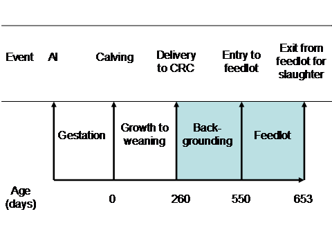
Slaughtering and post-slaughter inputs are omitted from this study. However, Johnston et al. (2003b, p. 136) reported that considerable effort was made to standardise these inputs. Also, animals were subject to similar backgrounding prior to entry to the feedlot. All animals were received by the Beef CRC as weaners prior to backgrounding. Variations occur in physical characteristics among animals of the same breed entering the backgrounding stage due to herd-of-origin effects brought about by differences between cohorts in sires and dams, and seasonal conditions in the pre-weaning stage. Figure 1 gives the timetable for preparing cattle to Korean market standards. The shaded area shows the period during which the cattle were under the control of the Beef CRC management.

Figure 1. Timetable for preparing lot-fed cattle to the Korean market standards

Four output variables are included in the analysis: amount of carcass weight produced, proportion of carcass weight retained after cooking, meat quality and marbling. The amount of carcass weight produced is measured as hot carcass weight in kilograms. The proportion of carcass weight retained after cooking was derived from a variable reported by Reverter et al. (2003b, p. 151) as cooking loss percentage. Because it is desirable for output variables in a production function to have positive relations with inputs, retention weight after cooking was calculated as a percentage by subtracting cooking loss percentage from 100.

A composite index of four sensory measures of quality was used to measure the quality of meat output. Johnston et al. (2003b, p. 137) termed this variable the sensory MQ4 score, including tenderness, juiciness, flavour and overall acceptability scores ^[1]. Because of the very high correlations among all of these four individual scores (Johnston et al., 2003b, p. 143), we expect to lose little information by using the composite index rather than four individual meat quality variables.

Two alternatives were available to represent the marbling of meat: the proportion of intramuscular fat and a discrete marbling score specified by AUS-MEAT (1998). The former was preferred because it is a continuous variable.

3. Model specification

We use a multi-input multi-output stochastic input distance function (Coelli and Perelman 1996, Coelli and Fleming 2005) to calculate technical efficiency indices for each sampled lot-fed animal, mean technical efficiency for each breed and mean technical efficiency across all animals. A stochastic input distance function is used rather than the standard stochastic production function to accommodate the specification of more than a single output. The eight inputs in the model are feed intake, number of days in the feedlot, age, liveweight, muscle score, rib fat depth, rump fat depth and eye muscle area. The four outputs are carcass weight, meat quality, retention of weight and marbling.

Zero-one dummy variables are included in the distance function for year, heifer and breed. As the data observations spanned 1996 and 1997, a 1997 dummy variable is also included to test for any difference in productivity between years. The details of this model are provided in Appendix A for interested readers.

4. Estimates of production relations

4.1 Input-output relations

Estimates of input and output elasticities from the maximum-likelihood estimation of the stochastic input distance function model and their standard errors are presented in Table 2. We are particularly interested in the output elasticities, which are the coefficients of the input variables in the estimated model. They measure the percentage increase in all outputs for a one per cent increase in the use of each of the inputs. The sum of the estimated elasticities of the input variables is 0.78, so given the restriction required for homogeneity of degree +1 in inputs, the implied output elasticity for the omitted variable, age of the animal when entering the feedlot, is 0.22. Individual likelihood ratio tests on each input and output showed that all but one input and one output contribute significantly in model estimation.^[2]

Table 2. Estimates of the Input and Output Elasticities

Variable	Estimated elasticity	Standard error	t-value
Inputs:
Feed per day	0.10	0.010	9.99
Days in feedlot	0.53	0.0092	57.62
Liveweight	0.10	0.021	4.90
Rib fat depth	0.0080	0.0035	2.26
Rump fat depth	-0.0024	0.0039	-0.61
Eye muscle area	0.015	0.011	1.36
Muscle score	0.022	0.010	2.28
Outputs:
Carcass weight	-0.237	0.014	-16.56
Weight retention	-0.252	0.040	-6.26
Meat quality	0.014	0.006	2.20

The number of days in the feedlot is highly significant and has the highest elasticity at 0.53. Other elasticities estimated to be significantly greater than zero are daily feed intake and weight on entering the feedlot (each 0.10), muscle score (0.02), eye muscle area (0.015) and rib fat depth (0.01). Only the estimated coefficient for the rump fat depth variable is insignificantly different from zero. The elasticities of the animal characteristics are low, but these characteristics are virtually costless to maintain once they are established, in contrast to conventional inputs that need to be applied each year.

Coefficients on the two output variables, carcass weight (-0.237) and proportion of meat weight retained after cooking (-0.252), are negative, as expected, and highly significant at less than one per cent significance level. They reflect a positive impact of the set of input variables on these two outputs: a 10 per cent increase in all inputs would increase carcass weight by 2.4 per cent and the proportion of meat weight retained after cooking by 2.5 per cent. The significant and positive coefficient on the meat quality output variable was not expected. It indicates that the set of inputs as a whole have a negative impact on meat quality, although the small size of the estimated elasticity (0.014) suggests the magnitude of this impact is not very great. A possible explanation of this unexpected result is that the high correlation between meat weight retention and meat quality, and the highly significant impact of inputs on the former, is masking the true impact of inputs on meat quality. The marbling output variable (intramuscular fat percentage) was found not to be significantly influenced by the set of inputs ^[3]. A likelihood ratio test revealed that its omission from the estimated model had no significant effect and it is not reported in the results in Table 2.

4.2 Breed, heifer and year effects on productivity

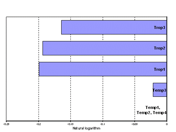
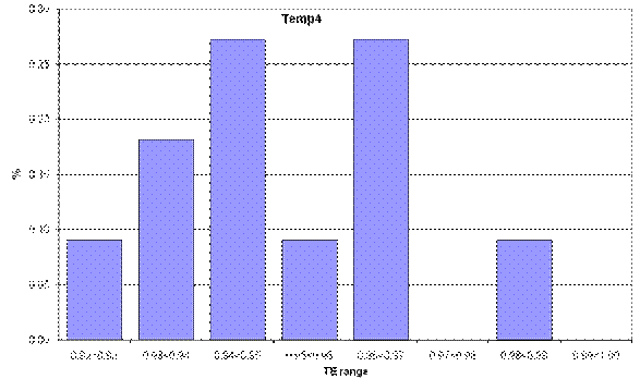
Individual likelihood ratio tests were conducted on the breed, year and heifer dummy variables in the distance function. In relation to breeds, Figure 2 shows the production frontiers of each breed of cattle in the sample. The frontiers of Temp1, Temp2 and Temp4 cattle are furthest from the origin (most productive). They are insignificantly different from each other, although it proved difficult to exactly place the frontier for Temp4 cattle given their small number of observations.

The frontier of Temp3 cattle is slightly but significantly below that for these three breeds (its scale parameter is 2.1 per cent less than that of the frontier breeds). The frontiers of the three tropically adapted breeds are much lower than the frontiers of the temperate breeds (scale parameters are lower than frontier breeds by 15.2 per cent for Trop3, 17.6 per cent for Trop2 and 18.1 per cent for Trop1).

A significant and positive coefficient for the 1997 year dummy variable indicates that feedlot productivity was higher in that year than in 1996. A significant and negative coefficient for the heifer dummy variable indicates that tropical heifer productivity is lower than steer productivity. The effect of this dummy variable is to reduce the scale parameter for heifers to around 2 per cent less than the parameter for steers.

Figure 2. Comparison of production frontiers by breed

Frontier differences

5. Technical inefficiency estimates

5.1 Evidence of technical inefficiency

The value of the test statistic for the null hypothesis of no technical inefficiencies of production (96.65) was found to be greater than the critical value obtained from Table 1 of Kodde and Palm (1986) for eight restrictions (14.85). We thus conclude that the technical inefficiency term (u_i in equation 1) is a significant addition to the model. A likelihood-ratio test that the coefficients on the breed efficiency variables are zero is strongly rejected, indicating that these variables as a group contribute significantly to an explanation of technical inefficiency in lot-fed beef production.

The gamma value (in equation 1), reflecting the percentage of error due to inefficiency, is not significantly different from unity, indicating that all residual variation is attributable to inefficiency and the random error is negligible. The lack of random effects reflects the strong control that managers have over the production environment in feedlot operations.

5.2 Influence of breed on technical inefficiency

The distance that cattle are located away from the frontier is likely to be influenced by variations in production potential among progeny from different sires and recent advances in breeding technology. It is proposed that performance is more tightly grouped (the mean technical efficiency index is higher) among breeds where the progeny come from a small pool of sires and the breed has not experienced substantial genetic advances in recent years.

These propositions are tested by including six breed dummy variables in the inefficiency effects model. The seventh breed, which is Temp1, is treated as the base. Given that Temp1 progeny come from the widest pool of sires that have experienced considerable recent genetic advances, it is expected that the signs on the coefficients of the six breed dummy variables will be negative, indicating lower technical inefficiency than Temp1.

All z-variables included in Table 3 except two contribute significantly (jointly and individually) to the explanation of technical inefficiencies in feedlot beef production. The Temp4 and Trop3 dummy variables are the exceptions (with both failing at the 5 per cent significance level).

Table 3. Estimates of the Efficiency Model

Variable	Estimated coefficient	Standard error	t-value
Constant	0.041	0.0046	8.81
Temp2 dummy variable	-0.017	0.0087	-1.93
Temp3 dummy variable	-0.048	0.0140	-3.41
Temp4 dummy variable	0.0084	0.0047	1.80
Trop1 dummy variable	-0.21	0.0217	-9.47
Trop2 dummy variable	-0.063	0.0161	-3.94
Trop3 dummy variable	-0.010	0.0080	-1.26
Sigma squared	0.00042	0.00002	24.99
Gamma	0.999	0.011	90.82

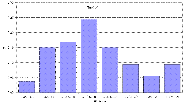
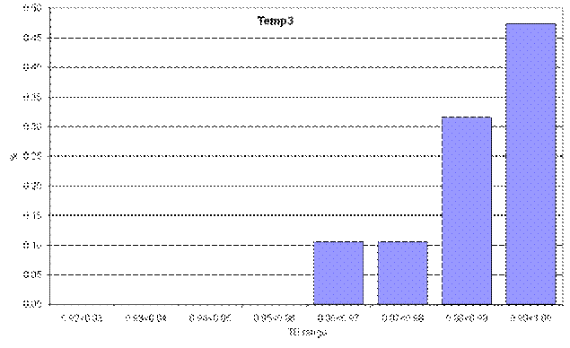
Plots of the distribution of the technical efficiency indices by breed are presented in Figure 3, with indices varying from 0.92 to 1.00. This is a narrow range but one to be expected given the controlled environment and identical management the animals receive from weaning through to slaughter. The high mean technical efficiency index indicates that a small but significant opportunity exists to increase beef output without using more physical and genetic inputs.

Figure 3. Distribution of technical efficiencies by breed

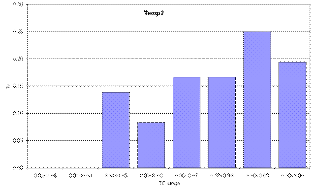
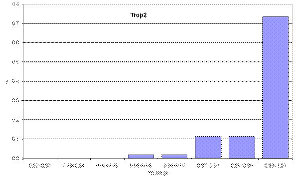
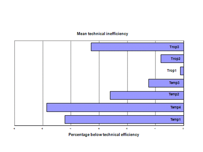
Controlling the quality of sires of progeny entering the feedlot is a way to raise technical efficiency. This point is illustrated in Figure 4. The mean technical efficiencies of each breed are to be interpreted relative to the frontier. Figure 4 shows the percentage by which the mean technical efficiency of each breed is less than perfect technical efficiency (100 per cent) (that is, below its frontier.

Figure 4. Comparison of mean technical efficiency indices across breeds

Trop1 cattle have the highest mean technical efficiency relative their own frontier (99.9 per cent), and Temp4 cattle have the lowest mean technical efficiency (95.1 per cent). A comparison of the results in Figure 2 and Figure 4 leads to the general observation that breeds with higher frontiers have lower mean technical efficiencies. Thus, breeding advances push the frontier upwards and this increases the variability in the breed performance (reflected by the lower mean technical efficiency score). The results for the Trop3 breed are slightly at odds with this observation.

Temp1 cattle come from most cohorts (and most sires), which would be expected to contribute to the relatively wide dispersion of technical efficiency indices for this breed. Temp4 cattle come from only two cohorts in one year but they have different pre-weaning backgrounds, resulting in a relatively wide dispersion of technical efficiency indices. The nature of their distribution, with few cattle near the frontier (Figure 3), suggests that our inability to specify a significant dummy variable for the breed in the estimated model has led to some frontier difference being picked up the breed dummy variable in the inefficiency effects model. Both Temp2 and Temp3 cattle have reasonably compact distributions of technical efficiency indices.

The tropically adapted breeds have fairly similar variations in cohorts, years and seasons in their samples but marked differences in spread of technical efficiency indices. Trop3 cattle have a much lower mean technical efficiency and wider distribution than Trop1 and Trop2 cattle, which is unlikely to be due solely to having one more cohort. Their mean technical efficiency is not significantly different from Temp1, Temp4 and Temp2 cattle.

In summary, the results of the inefficiency estimates accord with the proposition put forward earlier in this section about the effects of the width of the pool of sires and genetic advances on variations in technical efficiency indices. But further research is needed across a wider sample set to confirm these results.

6. Comparison of technical efficiency and feed use efficiency indices

Estimated technical efficiency indices were compared with the feed use efficiency indices calculated for each animal by the Cooperative Research Centre for Cattle and Beef Quality (Archer et al. 1998, Richardson et al. 1998). The latter indices were converted to indices between zero and unity by setting equal to unity the index of the most efficient animal in converting feed into weight gain. The feed use efficiency indices of other animals were set in proportion to this animal. The modified index provides a direct comparison with the technical efficiency index, with both indices lying between zero and unity. The purpose of the comparison is to assess how closely the partial measure of feed use efficiency compares with the more comprehensive technical efficiency index, which takes account of all inputs and outputs.

The correlation coefficient between technical efficiency indices estimated for each animal in the sample in this study with their corresponding feed use efficiency indices was estimated at +0.29. While there is a positive correlation between the indices, the quite low coefficient suggests that they are not close in measuring the efficiency of an animal in the production process. The feed use efficiency index measures how well an animal turns feed into weight gain. It therefore takes into account only one input and one output in the production process whereas the technical efficiency index measures all inputs and outputs. As important as the input of feed and output of weight gain are in the feed use efficiency index, their relationship is not sufficient to get an accurate picture of feedlot production efficiency.

7. Economies of diversification

7.1 Measuring diversification economies

The traditional economics text-book definition states that scope economies exist if a particular firm can produce two outputs at a lower cost than two separate firms specialising in the production of each of the two individual outputs. In this analysis, we investigate the existence of scope economies for two attributes of meat output. However, following Coelli and Fleming (2004), we call this measure, economies of diversification, which is derived from the second-cross partial derivatives of the estimated output distance function, to emphasise the distinction between it and the traditional economies of scope measure that is derived from a cost function. The measures are interpreted to mean that both attributes can be produced from one animal at a lower cost than it would take to produce the same levels of attributes from two animals that specialise to a greater degree in the production of one of the two attributes. The details of how this idea is implemented in a distance function framework are provided in Appendix B for interested readers.

7.2 Evidence of diversification economies

The coefficient estimates of diversification economies in the production system, defined in equation (6) of Appendix B, are reported in Table 4, for each pair of outputs at the means of the sample data. In order to test the hypothesis that there are no diversification economies, we calculated standard errors for these measures of diversification economies using a Taylor series expansion. The relatively high estimated standard error for carcass weight and retention proportion indicates that we would be unable to reject the null hypothesis of no diversification economies (or diseconomies) between these two outputs at any normal level of significance. (Findings are similar for relations between intramuscular fat content and all other outputs.)

The estimated value for retention proportion and meat quality is highly significant and quite large, at 1.10, indicating considerable potential for diversification economies by producing animals for these two outputs. This result accords with the expectation that greater retention of juices in the meat after cooking renders it more flavoursome, more juicier and more tender.

Table 4. Estimates of Economies of Scope

Output pair	Estimated coefficient	Standard error	t-value
Carcass weight-Retention	-0.67	0.72	-0.93
Carcass weight-Meat quality	-0.15	0.054	-2.73
Retention-Meat quality	1.10	0.26	4.21

A significantly negative coefficient for carcass weight and quality indicates that a trade-off exists between producing animals for weight and for quality. This finding has important implications for feedlot managers. Given they are aiming to finish off cattle at a target carcass weight of 280 kg, keeping animals in the feedlot to heavier carcass weights could be at the expense of higher quality meat. An explanation that meat of temperate beef breeds with lower carcass weight tends to be preferred to that of larger tropically adapted breeds does not stand up to scrutiny because the average carcass weight of tropically adapted cattle in the sample is 274 kg compared with 278 kg for temperate cattle. A more detailed examination by breed, however, reveals that Trop3 cattle in the sample have easily the highest mean carcass weight among breeds of 302 kg, well above the target weight, and easily the lowest mean MQ4 score of 46.7 compared with a mean score of 58.9 for all other animals.

8. Conclusions and Implications

This study has provided information about input-output relations, technical inefficiencies and diversification economies in a beef cattle feedlot in Australia. A production frontier was estimated, and it was found that tropically adapted breeds are further from the frontier than temperate breeds. The shape of the frontiers provides interesting results. Diversification economies were found to exist between the proportion of meat retention after cooking and meat quality. Diversification diseconomies were found between carcass weight and meat quality, although we suspect the relationship between the two outputs could vary between breeds. Further analysis is needed to study this relationship within each breed before a definitive statement could be made about the presence of diversification diseconomies between carcass weight and meat quality.

Information provided on technical inefficiency among breeds indicates that a small but significant amount of technical inefficiency exists in feedlot production. This means that there is an opportunity to expand beef output by controlling the quality of sires of progeny entering the feedlot.

References

Archer, J.A., Arthur, P.F., Herd, R.M. and Richardson, E.C. (1998), “Genetic variation in feed efficiency and it’s component traits”, Proceedings of the 6th World Congress on Genetics Applied to Livestock Production 25, 81-84.

AUS-MEAT (1998), Handbook of Australian Meat, Aus-Meat, Brisbane.

Barwick, S.A. and Henzell, A.L. (1997), “BreedObject: The selection tool for use with BREEDPLAN”, In Conference Proceedings for the BREEDPLAN Expo, National Beef Recording Scheme & New England Agricultural Secretariat Pty Ltd, Armidale, 27-28.

Barwick, S.A. and Henzell, A.L. (1998), “BreedObject: Breeding objective and indexing software for beef breeding”, Proceedings of the 6th World Congress on Genetics Applied to Livestock Production 27, 445-446.

Battese, G.E., Rao, D.S.P. and O’Donnell, C.J. (2004), “A metafrontier production function for estimation of technical efficiencies and technology gaps for firms operating under different technologies”, Journal of Productivity Analysis 21, 91-103.

Burrow, H.M., Johnston, D.J., Barwick, S.A., Holroyd, R.G., Barendse, W., Thompson, J.M., Griffith, G.R. and Sullivan, M. (2003), “Relationships between carcass and beef quality and components of herd profitability in northern Australia”, Proceedings Association for the Advancement of Animal Breeding and Genetics 15, 359-362.

Coelli, T.J. (1996), A Guide to FRONTIER Version 4.1: A Computer Program for Stochastic Frontier Production and Cost Function Estimation, CEPA Working Papers No. 7/96, Department of Econometrics, University of New England, Armidale.

Coelli, T.J. and Fleming, E. (2004), "Diversification economies and specialisation efficiencies in a mixed food and coffee smallholder farming system in Papua New Gu inea" Agricultural Economics, 31, 229-239.

Coelli, T.J. and Perelman, S. (1996), Efficiency Measurement, Multi-Output Technologies and Distance Functions: With Application to European Railways, CREPP WP 96/05, Centre de Recherche en Economie Publique et Economie de la Population, Université de Liège.

Coelli, T.J., Rao, D.S.P. and Battese, G.E. (1998), An Introduction to Efficiency and Productivity Analysis, Kluwer, Boston.

Deller, S.C., Chicoine, D.L. and Walzer, N. (1988), “Economies of size and scope in rural low-volume roads”, Review of Economics and Statistics 70, 459-465.

Farrell, M.J. (1957), “The measurement of productive efficiency”, Journal of the Royal Statistical Society, Series A, Part 3 120, 253-290.

Fleming, E., Farrell, T., Villano, R. and Fleming, P. (2006), “Is farm benchmarking the new acceptable face of comparative analysis?”, Australasian Agribusiness Review, Volume 14, paper 12. Available at: http://www.agrifood.info/review/2006/Fleming-et-al.html

Griffith, G.R., Rodgers, H.J., Thompson, J.M. and Dart, C. (2009), “The aggregate economic benefits to 2007/08 from the adoption of Meat Standards Australia”, Australasian Agribusiness Review 17, paper 5.

Available at: http://www.agrifood.info/review/2009/Griffith_Rodgers_Thompson_Dart.pdf

Grosskopf, S., Margaritis, D. and Valdmanis, V. (1995), “Estimating output substitutability of hospital services: a distance function approach”, European Journal of Operational Research 80, 575-587.

Johnston, D.J., Reverter, A., Burrow, H.M., Oddy, V.H. and Robinson, D.L. (2003a), “Genetic and phenotypic characterisation of animal, carcass and meat quality traits from temperate and tropically adapted beef herds: 1. Animal measures”, Australian Journal of Agricultural Research 54, 107-118.

Johnston, D.J., Reverter, A., Ferguson, D.M., Thompson, J.M. and Burrow, H.M. (2003b), “Genetic and phenotypic characterisation of animal, carcass and meat quality traits from temperate and tropically adapted beef herds: 3. Meat quality traits”, Australian Journal of Agricultural Research 54, 135-147.

Kodde, D.A. and Palm, F.C. (1986), “Wald criteria for jointly testing equality and inequality restrictions”, Econometrica 54, 1243-1248.

Newman, C. and Matthews, A. (2007), “Evaluating the productivity performance of agricultural enterprises in Ireland using a multiple output distance function”, Journal of Agricultural Economics 58(1), 128-151.

Reverter, A., Johnston, D.J., Perry, D., Goddard, M.E. and Burrow, H.M. (2003a), “Genetic and phenotypic characterisation of animal, carcass and meat quality traits from temperate and tropically adapted beef herds: 2. Abattoir carcass traits”, Australian Journal of Agricultural Research 54, 119-134.

Reverter, A., Johnston, D.J., Ferguson, D.M., Perry, D., Goddard, M.E., Burrow, H.M., Oddy, V.H., Thompson, J.M. and Bindon, B.M. (2003b), “Genetic and phenotypic characterisation of animal, carcass and meat quality traits from temperate and tropically adapted beef herds: 4. Correlations among animal, carcass, and meat quality traits”, Australian Journal of Agricultural Research 54, 149-158.

Richardson, E.C., Herd, R.M., Archer, J.A., Woodgate, R.T. and Arthur, P.F. (1998), “Steers bred for improved net feed efficiency eat less for the same feedlot performance”, Animal Production Australia, 22, 213-216.

Thompson, J., Polkinghorne, R., Watson, R., Gee, A. and Murison, R. (1998), “Meat Standards Australia, A 'PACCP' based beef grading scheme for consumers. 4) A cut based grading scheme to predict eating quality by cooking method”, Proceedings of the 45th International Congress of Meat Science and Technology, Yokohama, Japan. 45, 20-21.

Appendix A. Details of the Model Specification

We use a multi-input multi-output stochastic input distance function to calculate technical efficiency indices for each sampled lot-fed animal, mean technical efficiency for each breed and mean technical efficiency across all animals. Prior to estimation, the means of the log variables were adjusted to zero so that the coefficients of the first-order terms may be interpreted as elasticities, evaluated at the sample means.

Following Coelli and Perelman (1996), the translog stochastic input distance function used in this analysis can be defined as:

(1)

where X_m is the m-th input, Y_n is the n-th output, and a, b and w are parameters to be estimated. The eight inputs in the model are feed intake, number of days in the feedlot, age, liveweight, muscle score, rib fat depth, rump fat depth and eye muscle area. The four outputs are carcass weight, meat quality, retention of weight and marbling.

Zero-one dummy variables are included in the distance function for year, heifer and breed. As observations spanned 1996 and 1997, a 1997 dummy variable is included to test for any difference in productivity between years. The heifer dummy variable is included to test whether heifers are less productive than steers. Heifers comprised 35 of the 53 Trop2 cattle and 15 of the 26 Trop3 cattle whereas other breeds comprised solely steers. Hence, the heifer dummy will capture the effect of tropically adapted females rather than a generic female effect. The breed dummy variables are included to test whether different levels of genetic advance have been made between the seven breeds in the data set.

Again following Coelli and Perelman (1996), we set –ln d_I= v– u in equation (1) and impose the restriction required for homogeneity of degree +1 in inputs (Sβ_m = 1) to obtain the estimating form of the stochastic input distance function:

(2)

where A is the age of the animal; the vs are assumed to be independently and identically distributed with mean zero and variance, ; and the us are technical efficiency effects that are assumed to be truncated-normal and independently distributed such that u is defined by the truncation at zero of the normal distribution with unknown variance, s_u², and unknown mean, m, defined by:

(3)

where:

z₁ is the breed dummy variable for temperate breed 2 (Temp2);

z₂ is the breed dummy variable for temperate breed 3 (Temp3);

z₃ is the breed dummy variable for temperate breed 4 (Temp4);

z₄ is the breed dummy variable for tropically adapted breed 1 (Trop1);

z₅ is the breed dummy variable for tropically adapted breed 2 (Trop2); and

z₆ is the breed dummy variable for tropically adapted breed 3 (Trop3).

The variance parameters, s_v² and s_u², are replaced by g=s_u²/(s_v²+s_u²) and s_s²=(s_v²+s_u²) (Coelli and Perelman, 1996).

The input distances are predicted as:

d_i = E[exp(u) | e]

where e = v – u (Coelli and Perelman, 1996, p. 14).

Estimates of the parameters of the model were obtained using maximum-likelihood procedures in running the FRONTIER 4.1 program (Coelli, 1996). Various hypothesis tests were undertaken using likelihood-ratio tests, based on a 5 per cent significance level.

Appendix B. Measuring Scope/Diversification Economies

The traditional economics text-book definition states that scope economies exist if a particular firm can produce two outputs at a lower cost than two separate firms specialising in the production of each of the two individual outputs. In this analysis, outputs are produced as joint products of beef cattle. Therefore, all outputs must be produced to some extent and no choice exists for some outputs not to be produced at all. The combinations of outputs produced can be altered by genetic selection, by varying the proportions of different breeds in the herd or by varying the amounts of inputs used, such as feed per day and the number of days an animal spends in the feedlot. So here, scope economies for two attributes of meat output are interpreted to mean that both attributes can be produced from one animal at a lower cost than it would take to produce the same levels of attributes from two animals that specialise to a greater degree in the production of one of the two attributes. For example, managers of a feedlot would rather use animals that combine both high carcass weights and high-quality meat than have animals that yield a high carcass weight but produce meat of poor quality (or vice versa).

Consistent with the above definition, scope economies (implying cost complementarities) exist between outputs i and j if:

(4)

where C is the cost of N outputs and y_n is the n-th output variable (Deller, Chicoine and Walzer, 1988). The addition of an extra unit of output n reduces the marginal cost of producing an extra unit of output n’.

In this study, we estimate an input distance function instead of the traditional cost function because cost data do not exist for most inputs in the production system under study. We also allow for the possibility of inefficiency in production in the model.

Following Coelli, Rao and Battese (1998, p. 64), we define the input distance function as:

d (x,y) = {D: (x/D) L(y)}, (5)

where L(y) represents the set of all fixed and variable input vectors, x, that can produce the output vector, y. The expression, d(x,y), is non-decreasing in the input vector, x, increasing in the output vector, y, and linearly homogeneous and concave in x. The value of the distance function is equal to or greater than 1 if x is an element of the feasible input set, L(y). That is, d(x,y)≥1 if xL(y). It equals 1 if x is located on the inner boundary of the input set, where the firm is technically efficient, and exceeds 1 if the firm is technically inefficient. The input distance function value is therefore the inverse of the traditional input-oriented measure of technical efficiency, defined by Farrell (1957). We change the indices from the input distance function to conform to Farrell’s approach, inverting them so that they lie between 0 and 1.

The first partial derivative of the input distance with respect to the n-th output is negative. This sign indicates that the addition of an extra unit of output, holding all other variables constant, reduces the amount needed to put the observation onto the efficient frontier by deflating the input vector. A positive second cross partial derivative is evidence of economies of scope:

(6)

Conversely, a negative second cross partial derivative signifies diseconomies of scope.

^[1] These scores underpin the Meat Standards Australia voluntary beef grading scheme (Thompson et al. 1998, Griffith et al. 2009).

^[2] Similar test results were obtained for the standard normal tests associated with the t-values.

^[3] And at that time the Korean market was largely filled by grass-finished product, so marbling was not an important carcase characteristic.